Data Models and Query Languages (DDIA CH2)
Notes on chapter 2. of Designing Data-Intensive Applications.
Note: These notes were taken while reading chapter 2. of the book Designing Data-Intensive Applications, for more details please refer the book.
Table of Content
Most applications are built by layering one data model on top of another. each layer hides the complexity of the layers below it by providing a clean data model. Data models have a profound effect on what the software above can or can’t do.
Relational Model Versus Document Model
Relational Model (1980s) data is organised into relations (called tables in SQL), where each relation is an unordered collection of tuples (rows in SQL).
Driving forces behind the adoption of NoSQL (Non-relational databases) (2010s):
- Greater and easier scalability compared to Relational databases.
- Preference for free and open-source software.
- Specialised query operations.
- Restrictiveness of relational schemas, and a desire for a more dynamic and expressive data model.
Different applications have different requirements, best choice depends on the use case.
The Object-Relational Mismatch.
- Application development today is done in object-oriented programming languages.
- SQL stored data in relational models.
- A translation layer is required b/w them.
- Impedance mismatch: when two systems that are supposed to work together have different data models.
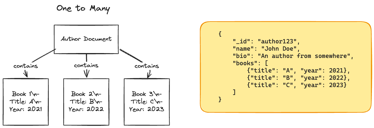
JSON Model.
- store it on a text column in the database, and let the application interpret its structure and content.
- Has better locality than multi-table schema.
- All the relevant information is in one place.
- In the relational model, you might need to query multiple tables or perform a multi-way join b/w different tables.
- Uses one-to-many relationships.
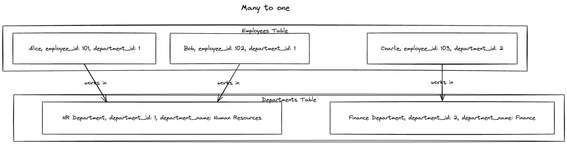
Many to one and Many to Many Relationships.
- For example, the name of a city stored in a database is standardised. There’s a city_id in the user table which maps to the city name in the city table. Advantages of this approach:
- Consistent style and spelling
- Avoiding ambiguity (In case of multiple cities by the same name)
- Easy to update in case the name of the city changes.
- Localisation support: if the site is translated, we can use the localised standardised list instead.
- Better search: Search all the users in the state.
- When we store text directly we are duplicating the human meaningful information for every record. But anything meaningful to humans may need to change sometime in the future. In case of duplication, all the redundant copies must be updated.
- Minimising redundancy in data is the key idea behind normalisation. (many to one)
- Many-to-one relationships don’t fit nicely into the document model, and support for joins is often weak.
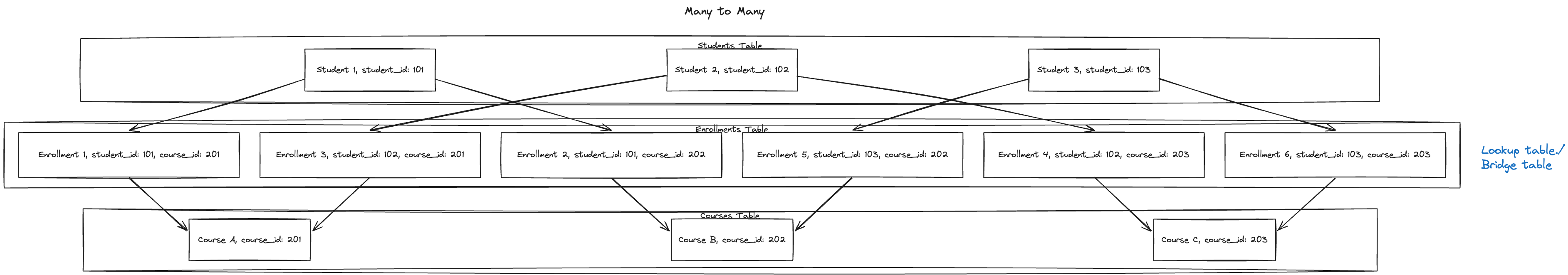
- relational databases also support many to many relationships. `
Relational Versus Document Databases Today
The main arguments in favour of the document data model are schema flexibility, better performance due to locality, and that for some applications it is closer to the data structures used by the application. The relational model counters by providing better support for joins, and many-to-one and many-to-many relationships.
Which data model leads to simpler application code?
Depends
- If the application has a document-like structure (tree of one-to-many relationships, where the entire tree is loaded at once.)
- We can’t refer directly to the nested item in a document-based database.
- Poor support for joining in the document database and not good for many-to-many relationships.
- It’s possible to reduce the need for join by denormalizing, but then the application code needs to do additional work to keep the denormalized data consistent.
- Joins can be emulated in application code by making multiple requests to the database, but that also moves complexity into the application and is usually slower than a join performed by specialized code inside the database.
- For highly interconnected data, the document model is awkward, the relational model is acceptable, and graph models (see “Graph-Like Data Models”) are the most natural.
Schema flexibility in the document model
Document databases are sometimes called schema-less, but that’s misleading, more accurate term is schema-on-read (the structure of the data is implicit, and only interpreted when the data is read), in contrast with schema-on-write (the traditional approach of relational databases, where the schema is explicit and the database ensures all written data conforms to it)
It’s Similar to discourse b/w static vs Dynamically typed languages.
When we want to change the format of the data
- Document: applications handle the cases for old and new data
- Relational: migration needs to be performed (Alter table)
Data locality for queries
- performance advantage to this storage locality.
- The locality advantage only applies if you need large parts of the document at the same time.
- Update operation: On updates to a document, the entire document usually needs to be rewritten—only modifications that don’t change the encoded size of a document can easily be performed in place
Convergence of document and relational databases
It seems that relational and document databases are becoming more similar over time, and that is a good thing: the data models complement each other. If a database can handle document-like data and also perform relational queries on it, applications can use the combination of features that best fits their needs.
- Most relational database systems (Other than MySQL) have supported XML since the mid-2000s. which allows applications to use data models very similar to what they would do when using a document database.
- Many database systems also have a similar level of support for JSON.
- Document databases like RethinkDB support relational-like joins in a query language.
Query Languages for Data
Imperative: tells the computer to perform certain operations in a certain order.
def getSharts():
	sharks = []
	for animal in animals:
		if animal.family == "Shark":
			sharks.append(animal)
	return sharks
Declarative query language Just specify the pattern of the data you want- what conditions the results must meet, and how you want the data to be transformed. But now how to achieve that goal.
Select * from animals where family = 'Shark';
Benefits:
- more concise and easier to work with
- database system can introduce performance improvements without requiring any changes to queries.
- declarative languages often lend themselves to parallel execution. database is free to use a parallel implementation of the query language, if appropriate
Declarative Queries on the Web
CSS: Declarative
li.selected > p {
    background-color: blue;
}
JavaScript: Imperative
var liElements = document.getElementsByTagName("li");
for (var i = 0; i < liElements.length; i++) {
    if (liElements[i].className === "selected") {
        var children = liElements[i].childNodes;
        for (var j = 0; j < children.length; j++) {
            var child = children[j];
            if (child.nodeType === Node.ELEMENT_NODE && child.tagName === "P") {
                child.setAttribute("style", "background-color: blue");
            }
        }
    }
}
- Much longer and harder to understand
- If the selected class is removed the attributions don’t revert back to normal (unlike CSS)
- Code needs to be updated to take advantage of new APIs
MapReduce Querying
- Neither declarative query language nor fully imperative query API. Somewhere in the middle.
- map(): aka collect, reduce() aka fold or inject.
Example: Generate a report of how many sharks you have sighted per months
SQL
SELECT date_trunc('month', observation_timestamp) AS observation_month,
       sum(num_animals) AS total_animals
FROM observations
WHERE family = 'Sharks'
GROUP BY observation_month;
MongoDB’s MapReduce (depreciated)
db.observations.mapReduce(
    function map() { // called once for every document which matches the query
        var year  = this.observationTimestamp.getFullYear();
        var month = this.observationTimestamp.getMonth() + 1;
        emit(year + "-" + month, this.numAnimals);
    },
    function reduce(key, values) { // runs for pairs with same key
        return Array.sum(values);
    },
    {
        query: { family: "Sharks" }, // filter is declarative (mongoDB specific)
        out: "monthlySharkReport" // final output is written to this collection
    }
);
MapReduce is a fairly low-level programming model for distributed execution on a cluster of machines.
Pros
- Can be run anywhere and re-run. (due to their specific nature)
- Powerful: they can parse strings, call library functions, perform calculations, and more.
Cons
- restricted, they must be pure functions and cannot perform additional database queries.
- Have to write two carefully coordinated JavaScript functions, which is often harder than writing a single query.
- A declarative query language offers more opportunities for a query optimizer to improve performance.
more about map-reduce in a later chapter.
Graph-like Data Models
- When many-to-many relationships are very common in your data.
- the relational model can handle simple cases, but when connections within your data become more complex, it becomes more natural to start modelling your data as a graph.
Graph
- Vertices: aka nodes aka entities
- Edges: aka relationships aka arcs
Homogeneous: when all the vertices represent the same kind of data. (Ex: People, Airport, WebPages etc.)
Heterogenous: Different types of objects in a single graph. (Ex: Facebook maintains People, location, events, checking and comments in a single graph)
Property Graph Model
In a property graph model, each vertex consists of:
- A unique id
- A set of outgoing edges
- A set of incoming edges
- A collection of properties (key-value pairs) Each edge consists of :
- A unique id
- the tail vertex
- the head vertex
- relationship b/w the two vertices
- A collection of properties (key-value pairs)
You can think of a graph store as consisting of two relational tables, one for vertices and one for edges.
CREATE TABLE vertices (
    vertex_id   integer PRIMARY KEY,
    properties  json
);

CREATE TABLE edges (
    edge_id     integer PRIMARY KEY,
    tail_vertex integer REFERENCES vertices (vertex_id),
    head_vertex integer REFERENCES vertices (vertex_id),
    label       text,
    properties  json
);

-- Indexes are created to speed up lookups for queries involving filters on tail index and head index
-- Ex: Select * from edges where tail_vertex == 1
-- This returns the set of outgoing edges to vertex 1

CREATE INDEX edges_tails ON edges (tail_vertex);
CREATE INDEX edges_heads ON edges (head_vertex);
Some important aspects of this model:
- Any vertex can have an edge connected with any other vertex
- Given any vertex, you can efficiently find its incoming and outgoing edges. (Indexes eges_tails and edges_heads have been created for this purpose)
- By using different labels we can store several different kinds of information in a single graph.
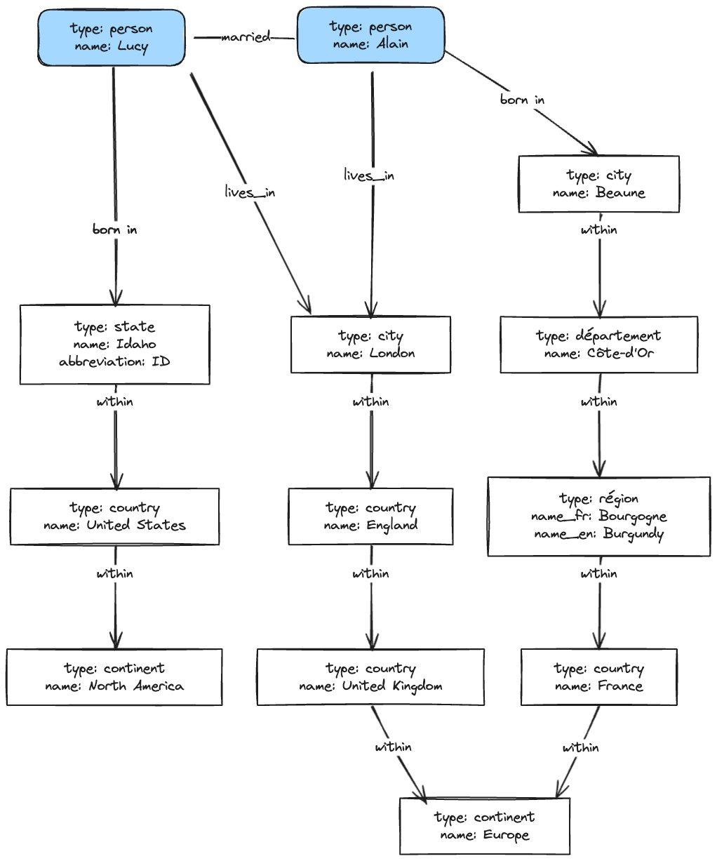
Things which would be difficult to express in a traditional relational schema
- Flexibility in structure (Different regional structures in different countries)
- Varying granularity of data (Lucy’s current residence is a city, where their birthplace is specified only at the state level.)
- Evolvability: as you add features to your application, a graph can easily be extended to accommodate changes in your application’s data structures.
The Cypher query language
A declarative query language for property graphs.
CREATE
  (NAmerica:Location {name:'North America', type:'continent'}), // vertex
  (USA:Location      {name:'United States', type:'country'  }),
  (Idaho:Location    {name:'Idaho',         type:'state'    }),
  (Lucy:Person       {name:'Lucy' }),
  (Idaho) -[:WITHIN]->  (USA)  -[:WITHIN]-> (NAmerica), // this defines the relationship b/w verte
  (Lucy)  -[:BORN_IN]-> (Idaho)
  // NAmerica, USA, Idaho, Lucy represent symbolic names (kind of like variables or constants)
Creates

Cypher query to find people who emigrated from the US to Europe
MATCH
  (person) -[:BORN_IN]->  () -[:WITHIN*0..]-> (us:Location {name:'United States'}),
  (person) -[:LIVES_IN]-> () -[:WITHIN*0..]-> (eu:Location {name:'Europe'})
RETURN person.name // return the name of the person matching above criteria

// () -[:WITHIN*0..] represents chasing of outgoing WITHIN edges
// It means following a WITHIN edge, zero or more times.
Equivalently, you could start with the two Location vertices and work backwards.
MATCH
  (us:Location {name:'United States'}) <-[:WITHIN*0..]- () <-[:BORN_IN]- (person),
  (eu:Location {name:'Europe'}) <-[:WITHIN*0..]- () <-[:LIVES_IN]- (person)
RETURN person.name
Graph Queries in SQL
We put graph data in a relational structure, can we also query it using SQL? Yes. But it’s messy. The same query had been written in cypher in 4 lines.
WITH RECURSIVE

  -- in_usa is the set of vertex IDs of all locations within the United States
  in_usa(vertex_id) AS (
      SELECT vertex_id FROM vertices WHERE properties->>'name' = 'United States'

      UNION

	  -- recursive step: traverse `WITHIN` relationships backwards
      SELECT edges.tail_vertex FROM edges
        JOIN in_usa ON edges.head_vertex = in_usa.vertex_id
        WHERE edges.label = 'within'
  ),

  -- in_europe is the set of vertex IDs of all locations within Europe
  in_europe(vertex_id) AS (
      SELECT vertex_id FROM vertices WHERE properties->>'name' = 'Europe'

	  UNION


	  -- recursive step: traverse `WITHIN` relationships backwards
      SELECT edges.tail_vertex FROM edges
        JOIN in_europe ON edges.head_vertex = in_europe.vertex_id
        WHERE edges.label = 'within'
  ),

  -- born_in_usa is the set of vertex IDs of all people born in the US
  born_in_usa(vertex_id) AS (
    SELECT edges.tail_vertex FROM edges
      JOIN in_usa ON edges.head_vertex = in_usa.vertex_id
      WHERE edges.label = 'born_in'
  ),

  -- lives_in_europe is the set of vertex IDs of all people living in Europe
  lives_in_europe(vertex_id) AS (
    SELECT edges.tail_vertex FROM edges
      JOIN in_europe ON edges.head_vertex = in_europe.vertex_id
      WHERE edges.label = 'lives_in'
  )

SELECT vertices.properties->>'name'
FROM vertices
-- join to find those people who were both born in the US *and* live in Europe
JOIN born_in_usa     ON vertices.vertex_id = born_in_usa.vertex_id
JOIN lives_in_europe ON vertices.vertex_id = lives_in_europe.vertex_id;
Triple-Stores and SPARQL
Mostly equivalent to the property graph model.
- All the info is stored in the form of three-part statements: (subject, predicate, object)
- The subject is equivalent to a vertex
- The object can be one of two things:
- A value in a primitive datatype. (predicate ~ key and object ~ value)
- Another vertex in a graph. (predicate ~ edge(edge_lable), object ~ head_vertex, subject~ tail_vertex)
Example: written as triples in a format called Turtle, a subset of Notation3 (N3)
@prefix : <urn:example:>.
_:lucy     a       :Person. #defining
_:lucy     :name   "Lucy". # Type-1 assigning value
_:lucy     :bornIn _:idaho. # Type-2 creating an edge b/w two vertices.
_:idaho    a       :Location.
_:idaho    :name   "Idaho".
_:idaho    :type   "state".
_:idaho    :within _:usa.
_:usa      a       :Location.
_:usa      :name   "United States".
_:usa      :type   "country".
_:usa      :within _:namerica.
_:namerica a       :Location.
_:namerica :name   "North America".
_:namerica :type   "continent".

# vertices are represented as _:<name>
We can use semicolons to say multiple things about the same subjects.
@prefix : <urn:example:>.
_:lucy     a :Person;   :name "Lucy";          :bornIn _:idaho.
_:idaho    a :Location; :name "Idaho";         :type "state";   :within _:usa.
_:usa      a :Location; :name "United States"; :type "country"; :within _:namerica.
_:namerica a :Location; :name "North America"; :type "continent".

Martin Kleppman. Designing Data Intensive Applicatioms . Kindle Edition.
The semantic web
- triple-store data model is completely independent of the semantic web
- The idea behind the semantic web: Websites already publish information as text and pictures for humans to read, so why don’t they publish info as machine-readable data for the computer to read?
- The RDF was created with the intention of building a web of data. (more below)
- It fell off but a lot of good work came out of it. (Triples for example)
The RDF data model
The Resource Description Framework (RDF) was intended as a mechanism for different websites to publish data in a consistent format, allowing data from different websites to be automatically combined into a web of data. (a kind of internet-wide “database for everything”)
<rdf:RDF xmlns="urn:example:"
    xmlns:rdf="http://www.w3.org/1999/02/22-rdf-syntax-ns#">

  <Location rdf:nodeID="idaho">
    <name>Idaho</name>
    <type>state</type>
    <within>
      <Location rdf:nodeID="usa">
        <name>United States</name>
        <type>country</type>
        <within>
          <Location rdf:nodeID="namerica">
            <name>North America</name>
            <type>continent</type>
          </Location>
        </within>
      </Location>
    </within>
  </Location>

  <Person rdf:nodeID="lucy">
    <name>Lucy</name>
    <bornIn rdf:nodeID="idaho"/>
  </Person>
- The (subject, predicate, object) are often URIs. Example: `http://my-company.com/namespace#within or http://my-company.com/namespace#lives_in,
- The reason is that different people might attach different meanings to word within or lives_in. This way we won’t get conflict.
- The URL does not need to be resolvable it’s just a namespace.
- RSS 1.0 was built around RDF.
The SPARQL query language
- SPARQL Protocol and RDF Query Language, pronounced “sparkle.”
- Predates Cypher, Cypher pattern matching is borrowed from SPARQL so they look quiet similar.
- Does not distinguish b/w properties and edges.
PREFIX : <urn:example:>

# gives name of the people who were born in United States and live in Europe
SELECT ?personName WHERE {
  ?person :name ?personName.
  ?person :bornIn  / :within* / :name "United States".
  ?person :livesIn / :within* / :name "Europe".
}

# variables start with "?"
# does not distinguish b/w properties and edges

# declering a variable
?usa :name "United States".
The Foundation: Datalog
- much older than SPARQL or Cypher. (studied in 1980s)
- Provided fundamentals that later query languages build upon.
- Used in Datamoic.
- Casalog is a Datalog implementation for querying large datasets in Hadoop.
- Similar to triple-store model.
- Format predicate(subject, object)
name(namerica, 'North America').
type(namerica, continent).

name(usa, 'United States').
type(usa, country).
within(usa, namerica).

name(idaho, 'Idaho').
type(idaho, state).
within(idaho, usa).

name(lucy, 'Lucy').
born_in(lucy, idaho).
Querying
- we define rules/predicates (kind of like functions)
- A rule applies if the system can find a match for all predicates on the righthand side of the :- operator. When the rule applies, it’s as though the lefthand side of the :- was added to the database (with variables replaced by the values they matched).
- These rules can be re-used which might cope better if the data is complex.
within_recursive(Location, Name) :- name(Location, Name).     /* Rule 1 */

within_recursive(Location, Name) :- within(Location, Via),    /* Rule 2 */
                                    within_recursive(Via, Name).

migrated(Name, BornIn, LivingIn) :- name(Person, Name),       /* Rule 3 */
                                    born_in(Person, BornLoc),
                                    within_recursive(BornLoc, BornIn),
                                    lives_in(Person, LivingLoc),
                                    within_recursive(LivingLoc, LivingIn).

?- migrated(Who, 'United States', 'Europe').